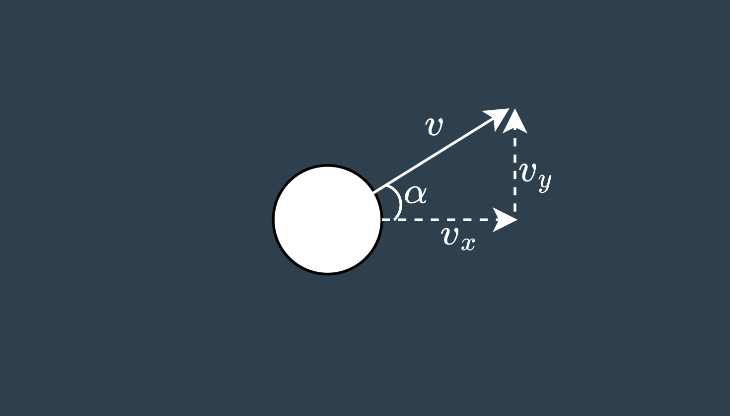
I should have mentioned it in part 1, but it is important that we are able to compute the ball path angle relative to the x-y plane at each time step. Since we will have the velocity vector for each step, we can compute this angle as follows

$$\alpha = \arctan(v_y / v_x)$$

Initial Conditions

It's important to define initial conditions for the problem. You can think of these as step 0, which we will use to find step 1. You have to start somewhere!

The things that we are solving for using previous states in the problem are

• launch angle This will be a user provided variable. Some common golf ball launch angles from a golf ball are about 5 degrees to 40 degrees.

• position This one is easy. We will say that the initial location of our golf ball is at the origin of the x,y plane (0,0)

• velocity Velocity is another user defined variable. We can use basic trigonometry to decompose the magnitude of our velocity into x and y components.

• acceleration It's not very intuitive, but we are going to simplify acceleration in this case and say we only have acceleration due to gravity and no lift or drag acceleration. In reality, we should be computing drag and lift at step 0 because the ball has non-zero velocity, but it will make a negligibly impact on our simulation.

Simulation Approach

Euler's Method

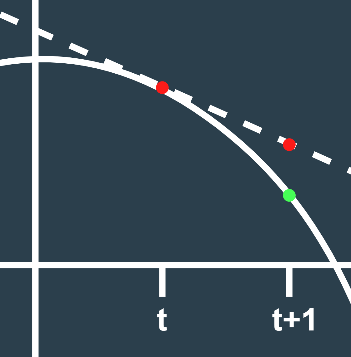
We will be using Euler's Method to compute each step in our simulation. To explain Euler's method in simple terms, imagine the below plot is a golf ball trajectory. We don't know the position at future points in time (t+1), but we know the velocity at the current point in time (dotted line @ t). Thus, we assume the velocity stays relatively constant between t and t+1.

In the case of this plot, the slope of the line changes dramatically between t and t+1, but our large time step is meant to exaggerate be an exaggeration. As time steps t and t+1 converge closer and closer together, our assumption of a constant velocity becomes better and better.

We'll use Euler's Method to solve for velocity and postion at the next time step in each step of our simulation. We'll use the current velocity and acceleration (time = t), to compute these future position and velocity (time = t+1) values.

$$dt = t - (t+1)$$ $$v_{t+1} = v_t + a_t * dt$$ $$x_{t+1} = x_t + v_t * dt$$

Parameters

Some important parameters to define in numerical integration include

Time step (dt) - Choosing this parameter is a balance between having sufficient fidelity in our model and not wasting compute for minimal fidelity gains. In this case, we can intuitively say that we should have somewhere on the order of 100 - 1000 time steps / second.

Simulation time - How long should my simulation run? In this case, we can intuitively think of an appropriate time. A golf ball would likely not be in the air for longer than 8 - 12 seconds, so we can set our run time to 12 seconds to be safe. ( Ultimately, we will stop the simulation when the golf ball "hits the ground" or the y-component of position falls below 0.)

Simulation Steps

So, here is what each step of our simulation will look like

1. Compute magnitude of the velocity vector

$$V = \lvert{v} = \sqrt{\square{v_x} + \square{v_y}}$$

2. Compute Reynolds Number

$$Re = \frac{{VD}}{{v}}$$

3. Compute Drag Coefficient

$$C_D = \begin{cases} 1.29 \times 10^{-10} \times \text{Re}^2 - 2.59 \times 10^{-5} \times \text{Re} + 1.50, & \text{if } \text{Re} < 10^5 \\ 1.91 \times 10^{-11} \times \text{Re}^2 - 5.40 \times 10^{-6} \times \text{Re} + 0.56, & \text{if } \text{Re} \geq 10^5 \end{cases}$$

4. Compute acceleration due to drag

$$a_D = \frac{{\rho V^2 A C_D}}{{2 m}}$$

5. Compute non-dimensional spin factor

$$S = \frac{{\omega r}}{{V}}$$

6. Compute lift coefficient

$$C_L = -3.25 S^2 + 1.99 S$$

7. Compute acceleration due to lift

$$a_L = \frac{{\rho V^2 A C_L}}{{2 m}}$$

8. Compute ball trajectory angle

$$\alpha = \arctan(\frac{{v_y}}{{v_x}})$$

9. Compute acceleration components in the x,y plane

$$a_x = -a_D * \cos(\alpha) - a_L * \sin(\alpha) a_y = -a_D * \sin(\alpha) + a_L * \cos(\alpha) - g$$

10. Compute velocity at the next time step

$$v_{t+1} = v_t + a_t * dt$$

11. Compute position at the next time step

$$x_{t+1} = x_t + v_t * dt$$

That's it! At each time step, we will save our position and velocity data in a state history array, and at the end we can plot our history.

In Part 3, we will implement these concepts in python and run a simulation.